Noise harassment—whether from persistent loud neighbors, industrial operations, or environmental disturbances—can have serious impacts on health and well-being. Chronic exposure to unwanted sound is linked to stress, anxiety, insomnia, and reduced concentration.
While traditional noise complaints rely on subjective reporting, advances in airborne acoustic monitoring now provide a precise, verifiable way to identify and document noise harassment events.
What Is Airborne Acoustic Monitoring?
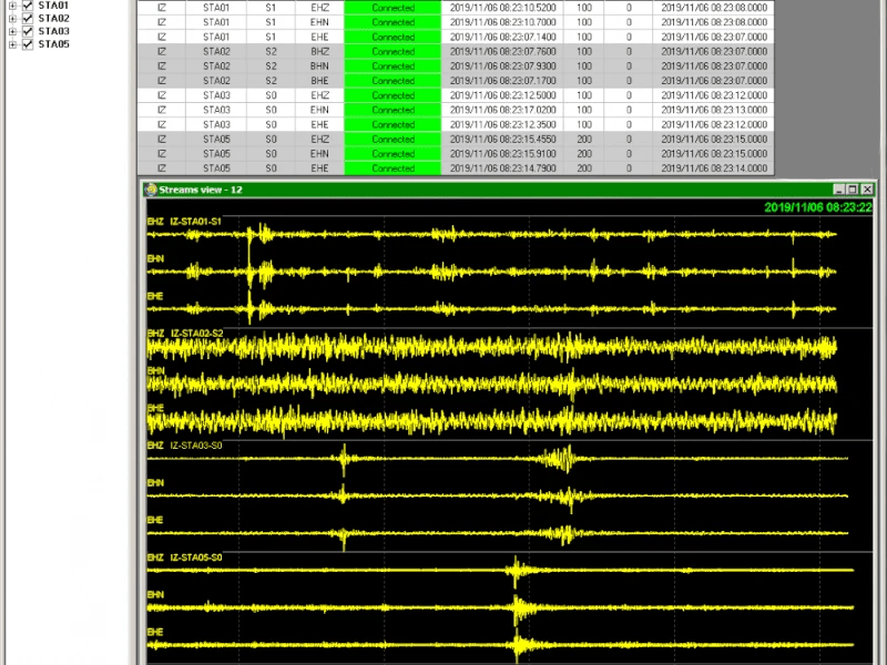
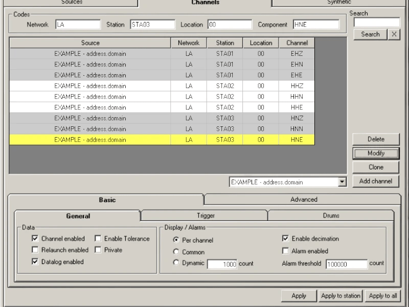
Airborne acoustic monitoring is the process of capturing and analyzing sound waves traveling through air using highly sensitive microphones and sensors. Unlike simple sound level meters, these systems:
- Continuously record noise levels in real time.
- Detect specific patterns and frequencies associated with harassment or nuisance sounds.
- Store and analyze historical data, creating a digital record for verification.
This makes the technology particularly useful for communities, workplaces, and legal authorities dealing with ongoing noise disputes.
Why Use Acoustic Monitoring for Noise Harassment?
1. Objective Evidence
Instead of relying solely on personal accounts, acoustic monitoring provides time-stamped, quantifiable data on noise events.
2. Continuous Surveillance
Systems can run 24/7, ensuring no event goes undocumented, even at night when disturbances are most disruptive.
3. Pattern Recognition
Advanced software can differentiate between normal background noise and intentional harassment, including:
- Repetitive banging or thumping
- High-frequency tones designed to irritate
- Amplified music or speech targeted at neighbors
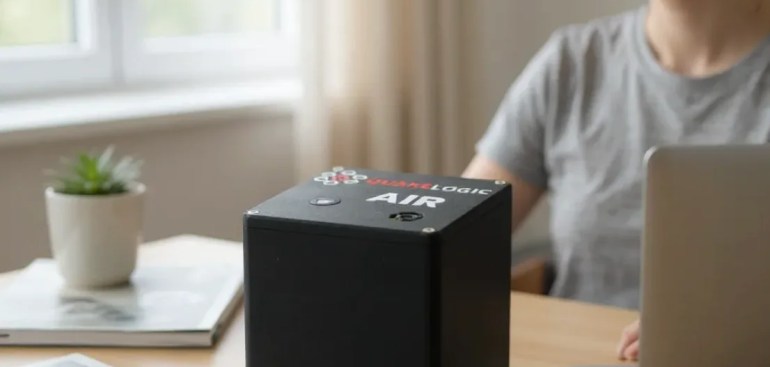
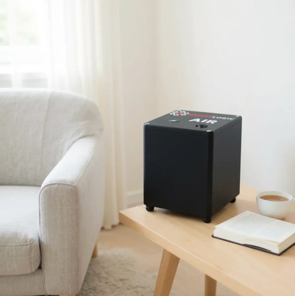
Introducing the QuakeLogic AIR Infrasound Monitor
For clients seeking a professional-grade solution, QuakeLogic proudly offers the AIR Infrasound Monitor. This advanced system is purpose-built for detecting and analyzing both audible noise and infrasound (below human hearing range), making it uniquely powerful for identifying subtle or intentionally disruptive harassment sources.

Key Advantages of AIR
- High-precision infrasound detection to capture low-frequency signals often missed by conventional microphones.
Whether for residents facing noise harassment, municipalities enforcing regulations, or industries monitoring compliance, AIR provides verifiable data.
Why QuakeLogic?
At QuakeLogic, we specialize in advanced monitoring solutions for seismic, vibration, and acoustic. Our AIR Infrasound Monitor represents the cutting edge of noise harassment detection—bridging the gap between traditional sound level meters and intelligent, cloud-connected monitoring systems.
Conclusion
Noise harassment is more than an inconvenience—it’s a public health issue. With the right tools, individuals, communities, and organizations can detect, document, and resolve noise disputes effectively. QuakeLogic’s AIR Infrasound Monitor transforms subjective complaints into actionable evidence, empowering a healthier, quieter future.
👉 Take control of your environment today. Explore the AIR Infrasound Monitor and empower your community with the evidence needed to ensure a healthier, quieter future.