Revolutionizing Earthquake Safety for Industrial and Commercial Systems
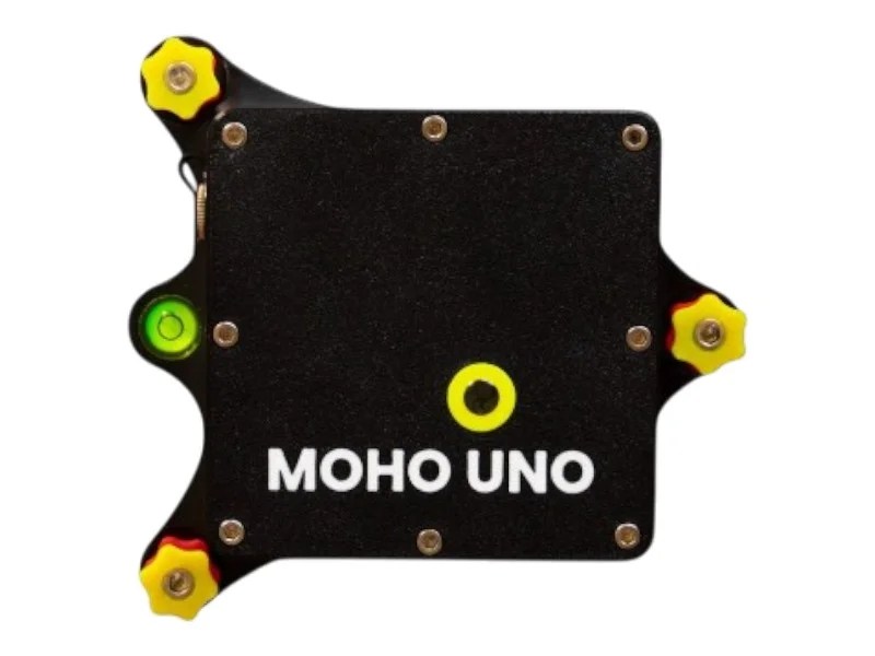
In a world where every second counts, QuakeLogic’s SATURN Series Smart Seismic Switch delivers instant earthquake detection and control designed to protect critical infrastructure and operations. Built on cutting-edge digital sensing technology, SATURN offers unmatched reliability, precision, and compliance — setting a new benchmark for seismic safety automation.


Intelligent Detection. Instant Protection.
The SATURN Series uses an advanced solid-state tri-axial seismic sensor to continuously monitor ground acceleration (PGA) in three dimensions (X, Y, and Z). When an earthquake occurs, the system instantly detects both P-waves and S-waves, calculates seismic intensity, and triggers connected safety mechanisms such as:
- Equipment and motor shutdowns
- Elevator recalls to safe floors
- Door and solenoid control
- Facility-wide alarm or PA notifications
This intelligent, plug-and-play seismic switch ensures your operations are protected automatically — even when power is disrupted, thanks to its integrated battery backup and external charger.
Built for Harsh Environments and Critical Infrastructure
Engineered to perform in demanding industrial and commercial settings, SATURN is the ideal solution for:
- Control rooms and manufacturing facilities
- Refineries, power plants, and water treatment plants
- Rail systems, data centers, and hospitals
- OEM integrations and automation systems
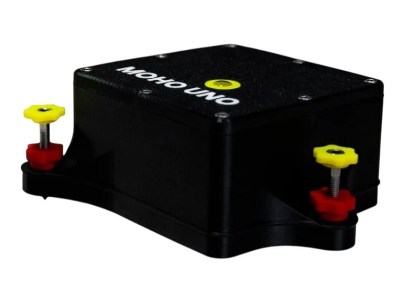
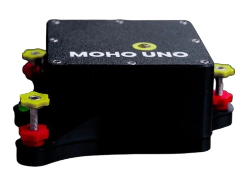
The unit’s rugged aluminum housing, sealed electronics, and false-trigger immunity make it highly resistant to noise from heavy machinery, compressors, trains, or elevators.
Compliance You Can Trust
The SATURN Series fully complies with leading safety and engineering standards — including UL 508, ASCE 25-97, ASME A17.1, and CA3137.
It meets the strict requirements for industrial control panels, elevator seismic shutdowns, and critical facility protection, making it a trusted solution for safety-critical applications worldwide.
Smart Integration and Flexibility
Each SATURN Seismic Switch features:
- Three Form-C relay outputs with dry, isolated contacts
- User-selectable trigger levels to match local seismic codes
- Configurable reset modes — manual latch or automatic timed trip (1–60 seconds)
- Internal terminal block for simple wiring and installation
Whether you’re integrating it into a new automation system or retrofitting an existing network, SATURN ensures seamless performance and peace of mind.
Data That Drives Decisions
Beyond triggering safety mechanisms, SATURN records XYZ peak ground acceleration (PGA) data in g-force, giving engineers and operators valuable insight into event intensity and system performance.
🪐 Models and Options
Available Models
SATURN S-001
• Horizontal mount, NEMA 4 enclosure
• Integrated rechargeable battery and universal 110/220 VAC power adapter
• UL-certified for industrial and commercial installations
• Ideal for standalone operation or integration with facility safety systems
SATURN-EB
• Horizontal mount, NEMA 4 enclosure
• 24 VDC (10 W) external power input (no internal battery or adapter)
• Optimized for control panels and OEM integrations requiring DC supply
Optional Accessories & Upgrades
Vertical Wall-Mount Kit
• Converts the SATURN base configuration for vertical installation
• Includes mounting hardware and pre-drilled alignment template
Stainless-Steel Primary Enclosure (NEMA 4X)
• Enhanced corrosion resistance for harsh or outdoor environments
• Precision-machined housing with reinforced seals
Bypass Switch Assembly
• Enables temporary bypass of seismic trigger for maintenance or testing
• Front-panel mounted toggle with safety lockout feature
Stainless-Steel Secondary Enclosure (NEMA 4X)
• Factory-machined housing with baseplate cutout and ventilation ports
• Available in two enclosure sizes:
– 16 in × 16 in × 8 in
– 24 in × 24 in × 12 in
• Ideal for added environmental protection or multi-unit installations
Why Choose SATURN Series from QuakeLogic?
✅ Proven reliability under extreme conditions
✅ Fast, accurate, and maintenance-free operation
✅ Seamless industrial integration
✅ Built for NEC and UL compliance
✅ Designed and supported in the USA
Final Thoughts
The SATURN Series Smart Seismic Switch isn’t just an instrument — it’s an intelligent safeguard that keeps your people, systems, and operations protected during seismic events.
When every millisecond matters, SATURN delivers confidence through precision.