Rotational Seismology with Tellus-R Seismometer

For decades, seismology has been defined by three translational components—X, Y, and Z.

Yet earthquakes do more than shift the ground; they also twist it. These subtle rotational motions hold vital insights into how seismic waves travel, how structures respond, and how hazards can be better understood. This is the foundation of rotational seismology, a rapidly advancing field that’s reshaping earthquake science.

Why Rotational Seismology Matters

Adding rotational motion to traditional measurements unlocks a fuller picture of seismic activity:

  • Seismic wavefield analysis: enables accurate modeling of wave propagation, scattering, and shear wave splitting.
  • Structural health monitoring: reveals torsional building responses often missed by translational sensors.
  • Engineering applications: improves earthquake-resistant design and helps refine seismic codes.

By recording all six degrees of freedom (6-DOF), rotational seismology bridges the gap between theoretical models and real-world earthquake impacts.

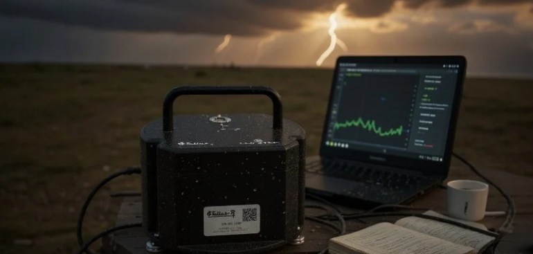
Tellus-R: Precision in Rotational Sensing

At the forefront of this movement is Tellus-R, a low-noise rotational seismometer built for both research and applied monitoring. It combines unmatched sensitivity, low power consumption, and rugged reliability.

Key Performance Highlights:

  • Resolution: 6×10⁻⁸ rad/s at 1 Hz
  • Dynamic range: 117 dB
  • Frequency range: 0.033–50 Hz (optional 0.01–100 Hz)
  • Noise floor: –125 dB (rel. 1 rad/s² Hz)
  • Power consumption: 30 mA at 10–18 VDC
  • Calibration input: optional 1:1 verification channel

Tellus-R’s hard-coated anodized aluminum body (IP67/IP68) ensures protection against harsh environments. Compact (Ø180 mm × 140 mm, 2 kg) yet robust, it operates in any orientation across temperatures from –15 °C to +55 °C (–40 °C optional).

Applications Across Science and Engineering

  • Earthquake research: capturing full 6-DOF motions near seismic sources
  • Structural engineering: studying torsional dynamics in bridges, towers, and dams
  • Seismic arrays: enhancing data from permanent and temporary networks
  • Geotechnical studies: advancing understanding of soil-structure interaction

Conclusion: Expanding the Future of Seismic Monitoring

Rotational seismology is redefining the way earthquakes are studied and structures are safeguarded. With its high precision, wide dynamic range, and field-proven durability, Tellus-R provides the critical measurements needed to push seismic science forward.

Seeing is Believing — explore how Tellus-R can revolutionize your seismic projects. Contact sales@quakelogic.net to learn more.


Choosing the Right Seismometer: Why One Size Doesn’t Fit All

Seismology and geophysical monitoring cover an enormous frequency spectrum — from the fast, high-frequency vibrations of a blast or building resonance to the slow “hum” of Earth itself. No single seismic sensor can capture this entire range with equal fidelity. That’s why different instruments exist, each optimized for a specific corner frequency, bandwidth, and application.

In this article, we explore when to use sensors with response corners at 4.5 Hz, 1 s, 2 s, 10 s, 30 s, 60 s, 120 s, and ultra-long 360 s, highlighting their strengths, weaknesses, and specific use cases. We also explain why one sensor cannot be used universally across all monitoring needs.


Quick Comparison of Seismic Sensors

Sensor TypeFrequency Range (Approx.)ProsConsTypical Applications
4.5 Hz Geophone4.5 Hz – 100+ HzLow cost, rugged, portable, sensitive to high frequenciesPoor at long-period (>1 s), limited dynamic rangeEarthquake engineering, structural monitoring, induced seismicity, aftershocks, MASW/ReMi, site surveys
1 s Sensor1 Hz – 50 HzGood compromise between local & regional coverage, handles ambient noiseLimited for very long-period (>30 s)Regional seismicity, volcano monitoring, EEW, ambient noise tomography, extended ReMi
2 s Sensor0.5 Hz – 50 HzCaptures regional & surface waves up to ~50 s, cost-effectiveInsufficient for very long-period (>100 s)Regional networks, subduction monitoring, passive seismic surveys
10 s Broadband0.1 Hz – 50 HzVersatile, reliable for most teleseismic and regional studiesCannot resolve very long-period oscillations (>120 s)National seismic networks, crustal/mantle imaging, hazard assessment
30 s Broadband0.03 Hz – 50 HzExtends into long-period surface wavesMore noise-sensitive, higher costGlobal seismology, tomography, moment tensor inversions
60 s Broadband0.016 Hz – 50 HzExcellent for large earthquake teleseisms, free oscillationsOverkill for regional/local studies, needs quiet vaultsGlobal networks, nuclear test monitoring
120 s Broadband0.008 Hz – 50 HzFull-spectrum coverage, ideal for global networksExpensive, requires special installationGSN stations, large earthquake research, planetary seismology
360 s Ultra-Broadband0.003 Hz – 50 HzCaptures Earth’s hum, seismic tides, geodynamicsNiche, very noise-sensitive, costlyGeodynamic observatories, tidal studies, climate-related mass transport

4.5 Hz Sensors (Short-Period Geophones)

When to use:

  • Local earthquake detection (within tens of kilometers).
  • Engineering and structural health monitoring.
  • Microseismicity, quarry or mine blasts.
  • Geophysical testing (MASW, ReMi, refraction/reflection).

Pros:

  • Rugged, portable, and low cost.
  • High sensitivity to high-frequency ground motions (>5 Hz).
  • Excellent for near-field strong-motion recording.

Cons/Limitations:

  • Poor sensitivity below ~1 Hz, cannot capture long-period seismic waves.
  • Unsuitable for regional and global/teleseismic events.
  • Limited dynamic range compared to broadband instruments.

Typical Applications:

  • Earthquake engineering, dam or bridge monitoring, induced seismicity, aftershock arrays.
  • Geophysical surveys such as MASW (Multichannel Analysis of Surface Waves for shallow Vs profiles), ReMi (Refraction Microtremor passive site characterization), and seismic refraction/reflection studies.

1 s Sensors

When to use:

  • Regional seismicity (hundreds of kilometers).
  • Strong-motion networks where both local and regional signals matter.
  • Volcano and microseismic monitoring.
  • Urban geophysical studies using ambient noise.

Pros:

  • Balanced response between short-period and moderate-period signals.
  • Captures both body waves and surface waves up to ~20–30 s.
  • Suitable for passive array surveys (extended ReMi, microtremor analysis).

Cons/Limitations:

  • Insufficient for very long-period (>30 s) surface waves.
  • Less sensitive to teleseisms than true broadband sensors.

Typical Applications:

  • Regional earthquake catalogs, EEW systems, volcano observatories.
  • Ambient noise tomography, urban microzonation, extended ReMi studies for deeper shear-wave velocity profiling.

2 s Sensors

When to use:

  • Regional to teleseismic earthquakes.
  • Arrays where both body and surface waves are important.
  • Cost-sensitive networks needing extended bandwidth.

Pros:

  • Wider bandwidth than 1 s, capable of recording surface waves up to ~50 s.
  • Good compromise between cost and performance.

Cons/Limitations:

  • Not sufficient for very long-period (>100 s) phenomena.
  • Still more noise-sensitive than longer-period broadband sensors.

Typical Applications:

  • Regional seismic monitoring, tectonic studies, subduction zone networks.
  • Passive seismic surveys requiring both regional and long-period information.

10 s Sensors

When to use:

  • General-purpose broadband seismic networks.
  • Regional and teleseismic earthquake detection.

Pros:

  • Industry standard broadband response.
  • Sensitive to both surface and body waves.
  • Reliable and versatile for many applications.

Cons/Limitations:

  • Cannot resolve very long-period (>120 s) free oscillations.

Typical Applications:

  • National networks, crustal imaging, mantle tomography.
  • Earthquake source characterization and hazard assessment.

30 s Sensors

When to use:

  • Long-period surface wave studies.
  • Subduction and mantle structure investigations.
  • Broadband observatories.

Pros:

  • Extends useful response to long-period surface waves.
  • Stable in low-noise environments.

Cons/Limitations:

  • Higher cost and more complex installation.
  • Susceptible to cultural and wind noise.

Typical Applications:

  • Tomography, global seismology, moment tensor inversion.

60 s Sensors

When to use:

  • Large earthquake teleseisms.
  • Long-period mantle and core phase recordings.

Pros:

  • Excellent for large-magnitude earthquakes.
  • Sensitive to Earth’s free oscillations.

Cons/Limitations:

  • Over-engineered for local or regional seismic monitoring.
  • Requires very quiet installation sites.

Typical Applications:

  • Global seismic networks, nuclear test monitoring, Earth structure studies.

120 s Sensors

When to use:

  • Global seismology, full spectrum earthquake monitoring.
  • Earth’s free oscillations and tidal studies.

Pros:

  • Covers almost the entire seismological band (0.008–50 Hz).
  • Critical for large, distant earthquakes.

Cons/Limitations:

  • Expensive, complex, vault installation needed.
  • Not practical for engineering-scale or high-frequency studies.

Typical Applications:

  • GSN (Global Seismographic Network), Earth structure research, planetary seismology.

360 s Sensors (Ultra-Long-Period Broadband)

When to use:

  • Recording Earth’s “hum” and seismic tides.
  • Geodynamic monitoring of slow, long-period processes.

Pros:

  • Extends response into tidal and ultra-long-period bands.
  • Captures signals invisible to conventional broadband sensors.

Cons/Limitations:

  • Highly sensitive to environmental noise.
  • Costly and niche, requiring ultra-quiet observatory conditions.

Typical Applications:

  • Geodynamics, glacial isostatic adjustment, climate-related mass transport studies.

Why One Sensor Can’t Do It All

  1. Frequency Trade-Offs: A sensor tuned for high-frequency microseismic signals cannot also detect Earth tides and free oscillations.
  2. Dynamic Range: Instruments designed for small ambient noise may clip during strong shaking.
  3. Installation & Cost: Ultra-broadband sensors need expensive vaults and isolation, while geophones are portable and inexpensive.
  4. Application-Specific Needs: Engineering, geophysics, regional monitoring, and global seismology each demand different spectral coverage.

Conclusion

The “best” seismic sensor depends on what you want to measure.

  • 4.5 Hz geophones dominate in engineering seismology, structural monitoring, MASW, ReMi, and site investigations.
  • 1–2 s sensors bridge the gap for regional seismicity and passive geophysical surveys.
  • 10–120 s broadband sensors are the backbone of national and global seismic networks.
  • 360 s ultra-broadband sensors are specialized tools for studying Earth’s slowest processes.

Seismology is broadband by nature, but practice demands choosing the right tool for the job.

At QuakeLogic, our experts can help you for selecting the right seismometer for your application.

To explore our range of seismometers, visit us at https://products.quakelogic.net/seismometers/

Galperin vs Orthogonal Seismometer Configurations: What’s the Difference and Why It Matters?

In seismic monitoring, triaxial seismometers are essential tools that capture ground motion in three dimensions. But not all triaxial sensors are designed the same way. Two dominant configurations exist: the orthogonal layout and the Galperin symmetric design. Understanding the difference between them is key when deciding how to choose a broadband seismometer or designing your seismic network.

Orthogonal Configuration: The Traditional Layout

Orthogonal seismometers use three sensing elements aligned at right angles:

  • X-axis (East-West)
  • Y-axis (North-South)
  • Z-axis (Vertical)

This configuration provides direct and intuitive measurements of ground motion along geographic axes. It is commonly found in strong-motion sensors and legacy seismic stations.

Pros:

  • Simple and direct mapping to geographic directions
  • Standard format for data processing
  • Useful in structural monitoring when orientation is controlled

Cons:

  • Requires precise alignment to true North and level installation
  • Uneven horizontal sensitivity
  • Prone to increased cross-axis coupling due to asymmetry

Galperin Configuration: The Modern Symmetric Design

First introduced by Evgeny Galperin, this configuration uses three identical sensors, each spaced 120° apart and tilted equally from vertical (typically ~35.26°). Rather than directly measuring along X, Y, and Z, these sensors capture intermediate components. Standard vertical and horizontal motion is then reconstructed through a simple mathematical transformation.

Galperin geometry forms the basis of modern broadband seismometers, including all broadband seismometers offered by QuakeLogic.

Pros:

  • Isotropic azimuthal sensitivity for uniform horizontal response
  • Mechanically balanced and compact design
  • Easier installation — no need for precise geographic orientation
  • Ideal for low-noise, high-fidelity broadband recording
  • Often includes self-leveling mechanisms

Cons:

  • Requires post-processing to derive standard components (Z, N, E)
  • May be unfamiliar to users expecting direct XYZ outputs

Coordinate Transformation in Galperin Systems

The raw sensor outputs (V1, V2, V3) from a Galperin layout are converted into vertical (Z) and orthogonal horizontal (X, Y or N, E) components through a transformation matrix. The result is functionally identical to orthogonal output — but with superior mechanical and dynamic performance.

To obtain standard seismic components — vertical (Z), north (N), and east (E) — from a Galperin-configured broadband seismometer, a mathematical transformation is applied to the raw outputs of the three equally tilted sensors.

Galperin sensors are mounted 120° apart in azimuth and tilted at approximately 35.26° from vertical. This symmetric geometry ensures equal sensitivity in all horizontal directions, making it ideal for high-fidelity broadband seismic recording.

The transformation to orthogonal components is handled by a fixed matrix derived from the Galperin geometry. Here’s a practical example in Python that demonstrates how to convert the raw Galperin outputs (V1, V2, V3) into Z, N, and E components:

import numpy as np

def galperin_to_orthogonal(V1, V2, V3):
    """
    Transforms Galperin outputs (V1, V2, V3) into orthogonal components (Z, N, E).
    
    Assumes Galperin sensors are tilted 35.26 degrees from vertical and 120 degrees apart in azimuth.
    """

    # Galperin angle in degrees and radians
    alpha_deg = 35.2643897  # approximately arccos(1/sqrt(3))
    alpha_rad = np.radians(alpha_deg)

    # Transformation matrix based on Galperin geometry
    # Source: Galperin 1985; commonly used form
    T = np.array([
        [np.cos(alpha_rad), np.cos(alpha_rad), np.cos(alpha_rad)],  # Z (vertical)
        [np.sin(alpha_rad), -0.5 * np.sin(alpha_rad), -0.5 * np.sin(alpha_rad)],  # N (North)
        [0, np.sqrt(3)/2 * np.sin(alpha_rad), -np.sqrt(3)/2 * np.sin(alpha_rad)]  # E (East)
    ])

    # Stack Galperin outputs into column vector
    V = np.array([V1, V2, V3])

    # Perform transformation
    Z, N, E = T @ V

    return Z, N, E

# Example usage
V1, V2, V3 = 0.1, 0.2, 0.15  # Example raw sensor outputs
Z, N, E = galperin_to_orthogonal(V1, V2, V3)

print("Vertical (Z):", Z)
print("North (N):", N)
print("East (E):", E)

This code is useful for researchers, engineers, or software developers integrating Galperin seismometers into their own data acquisition systems or post-processing pipelines.

Why Galperin Excels in Broadband Performance

Galperin-configured sensors offer lower cross-axis sensitivity, reduced internal noise, and azimuthal symmetry. This makes them particularly suited for high-precision seismological research.

Optimizing Your Network Design

Because Galperin-based instruments don’t require precise geographic orientation, they simplify field deployments and reduce installation error. This is especially helpful in large-scale projects and remote installations.

✅ QuakeLogic’s Seismometer Solution

At QuakeLogic, we exclusively offer Galperin-type broadband seismometers, engineered for superior sensitivity, symmetrical mechanical design, and fast, easy deployment. Our systems are:

  • Fully turnkey, with no licensing or calibration fees
  • Designed for broadband performance with low self-noise
  • Delivered with user-friendly software and optional remote monitoring tools
  • Compatible with standard seismic analysis workflows

Whether you’re deploying a temporary station or building out a national seismic network, Galperin configuration delivers the performance you need with the reliability you trust.

📞 Contact Us

Ready to upgrade your monitoring system? Reach out to our team at sales@quakelogic.net or browse our product line at products.quakelogic.net to explore QuakeLogic’s advanced broadband solutions.